
This is the second of a two-part series of blog posts focused on GHC’s specialization optimization. Part 1 acts as a reference manual documenting exactly how, why, and when specialization works in GHC. In this post, we will finally introduce the new tools and techniques we’ve developed to help us make more precise, evidence-based decisions regarding the specialization of our programs. Specifically, we have:
- Added two new automatic cost center insertion methods to GHC to help us attribute costs to overloaded parts of our programs using traditional cost center profiling.
- Developed a GHC plugin that instruments overloaded calls and emits data to the event log when they are evaluated at runtime.
- Implemented analyses to help us derive conclusions from that event log data.
To demonstrate the robustness of these methods, we’ll show exactly how we
applied them to Cabal to achieve a 30% reduction in run time
and a 20% reduction in allocations in Cabal’s .cabal file parser.
The intended audience of this posts includes intermediate Haskell developers that want to know more about specialization and ad-hoc polymorphism in GHC, and advanced Haskell developers that are interested in systematic approaches to specializing their applications in ways that minimize compilation cost and executable sizes while maximizing performance gains.
This work was made possible thanks to Hasura, who have supported many of Well-Typed’s initiatives to improve tooling for commercial Haskell users.
I presented a summary of the content in Part 1 of this series on The Haskell Unfolder. Feel free to watch it for a brief refresher on what we have learned so far:
The Haskell Unfolder Episode 23: specialisation
Overloaded functions are common in Haskell, but they come with a cost. Thankfully, the GHC specialiser is extremely good at removing that cost. We can therefore write high-level, polymorphic programs and be confident that GHC will compile them into very efficient, monomorphised code. In this episode, we’ll demystify the seemingly magical things that GHC is doing to achieve this.

Example code
We’ll begin by applying these new methods to a small example application that is specifically constructed to exhibit the optimization behavior we are interested in. This will help us understand precisely how these new tools work and what information they can give us before scaling up to our real-world Cabal demonstration.
If you wish, you can follow along with this example by following the instructions below.
Our small example is a multi-module Haskell program. In summary, it is a program containing a number of “large” (as far as GHC is concerned) overloaded functions that are calling other overloaded functions other across module boundaries with various dictionary arguments. The call graph of the program looks like this:

Specializable calls are labelled with their concrete type arguments. All
non-recursive calls are across module boundaries. Here is the code, beginning
with the Main module:
module Main where

import Types
import Value

main :: IO ()
main = do
    let
      !vInt = value @MyInt 100_000
      !vDouble = value @MyDouble 1_000_000
      !vIntegers = sum $ map (value @MyInteger) [1 .. 5_000]
    putStrLn "Done!"
The main function computes three values of different types by calling the
overloaded value function at those types, and then prints “Done!”. The
MyInt, MyDouble, and MyInteger types and are defined in the Types
module:
module Types where

data MyInt = MyInt !Int
  deriving (Eq, Ord)
instance Num MyInt where ...

data MyDouble = MyDouble !Double
  deriving (Eq, Ord)
instance Num MyDouble where ...

data MyInteger = MyInteger !Integer
  deriving (Eq, Ord)
instance Num MyInteger  where ...
instance Enum MyInteger where ...
We define these types and instances like this for subtle purposes of
demonstration1. The overloaded value function comes from
the Value module:
module Value where

import Divide
import Multiply

value :: (Ord n, Num n) => n -> n
value n = (n `multiply` 10) `divide` n
value makes overloaded calls to the multiply and divide functions from the
Multiply and Divide modules:
module Multiply where

import Plus

multiply :: (Eq n, Num n) => n -> n -> n
multiply x y
    | x == 0    = 0
    | otherwise = y `plus` ((x - 1) `multiply` y)
module Divide where
import Plus
divide :: (Ord n, Num n) => n -> n -> n
divide x y
| x < y = 0
| otherwise = 1 `plus` ((x - y) `divide` y)Finally, multiply and divide both make overloaded calls to plus from the
Plus module:
module Plus where

plus :: Num n => n -> n -> n
plus x y = x + y
Since we’ll be instrumenting this code with a GHC plugin later, we glue it together with this Cabal file:
cabal-version:   3.8
name:            overloaded-math
version:         0.1.0

executable overloaded-math
    default-language: GHC2021
    main-is:          Main.hs
    other-modules:    Divide, Multiply, Plus, Types, Value
    build-depends:    base
    ghc-options:
      -funfolding-creation-threshold=-1
      -funfolding-use-threshold=-1
We pass
-funfolding-creation-threshold=-1 and
-funfolding-use-threshold=-1 to simulate a
scenario where all of these bindings are large enough that no inlining will
happen by default.
If we spent enough time staring at this program, we might eventually figure out
that the path to plus through multiply is the “hot path”, because the
recursion in multiply advances much slower than the recursion in divide. The
calls on that path are thus our top candidates for specialization. It would take
even more staring, however, to determine exactly which specializations (which
functions at which types) will actually result in the biggest performance
improvement. In this specific case, specializing the calls to value,
multiply, and plus at the MyInteger type will result in the biggest
performance improvement. Let’s see how our new methods can help us come to that
exact conclusion without requiring us to stare at the code.
Dancing with the devil (a.k.a. the GHC specializer)
Recall the specialization spectrum from Part 1. Our goal is to systematically explore that spectrum and find our “ideal” point, striking a balance between performance and code size/compilation cost. However, before we can explore the spectrum, we need to bound the spectrum. In other words, we need to determine where our “baseline” and “max specialization” points are, so we can determine how much we actually have to gain from specialization.
Bounding the specialization spectrum
To characterise a given point on the specialization spectrum, we will measure the compilation cost, code size, and performance of the program at that point. Let’s start with the “baseline” point and measure these metrics for the code as it is right now, with no extra pragmas or GHC flags.
To measure compilation cost, we will pass the -s RTS flag to
GHC, which makes the runtime system of GHC itself output execution time and
allocation statistics:
cabal build overloaded-math --ghc-options="+RTS -s -RTS"Passing --ghc-options="+RTS -s -RTS" means cabal will pass +RTS -s -RTS
when it invokes GHC, so the output will be the runtime and allocation statistics
of the GHC compiling the program, not the program itself.
Note that cabal invokes ghc multiple times during a cabal build, and it
will supply the given --ghc-options options for each invocation. We are only
interested in the statistics resulting from the actual compilation of the
modules, so look for the output immediately following the typical [6 of 6] Compiling Main ... GHC output. The stats that we typically care most about are
bytes allocated, maximum residency, and total CPU time:
[6 of 6] Compiling Main             ( src/Main.hs, ...)
     243,729,624 bytes allocated in the heap
...
      11,181,432 bytes maximum residency (4 sample(s))
...
  Total   time    0.201s  ...
...
For more information on exactly what the numbers in this output mean, see the runtime system documentation in the GHC User’s Guide.
Let’s check the code size by measuring the size of the resulting object files.
Note that we should discard the Types module from our measurements, since it
only exists for demonstration. This can be done with something like the
following command:
ls dist-newstyle/**/*.o | grep -v Types | xargs du -bcThis command lists all object files in the dist-newstyle directory, removes
the Types module from the list, and passes the rest to the du command. The
-bc flags2 tell du to display the sizes in bytes and
output a sum of all sizes:
2552    .../Divide.o
4968    .../Main.o
2872    .../Multiply.o
1240    .../Plus.o
2048    .../Value.o
13680   total
Finally, we can measure performance of our actual program (not GHC) by running
our executable and passing the -s RTS flag:
cabal run overloaded-math -- +RTS -sWe’ll note the same statistics that we did when measuring compilation cost:
   3,390,132,896 bytes allocated in the heap
...
      36,928,976 bytes maximum residency (6 sample(s))
...
  Total   time    0.630s  ...
...
To collect all of these stats at the “max specialization” point of the spectrum,
we repeat the commands above, passing
-fexpose-all-unfoldings and
-fspecialize-aggressively as --ghc-options
in each of the cabal invocations.
Here is a summary of our results, with the compilation cost and performance metrics averaged over three samples. All sizes are in bytes and all times are in seconds:
| Metric | Baseline | Max specialization | Change |
|---|---|---|---|
| Code size | 13,680 | 23,504 | +72% |
| Compilation allocation | 243,728,331 | 273,619,112 | +12% |
| Compilation max residency | 11,181,587 | 19,864,283 | +78% |
| Compilation time | 0.196 | 0.213 | +8.7% |
| Execution allocation | 3,390,132,896 | 877,242,896 | -74% |
| Execution max residency | 36,928,976 | 23,921,576 | -35% |
| Execution time | 0.635 | 0.172 | -73% |
As expected, relative to our baseline, max specialization has increased code size and compilation cost and improved performance.
Whole program specialization
If you are following along, you may have
noticed that the module whose object file size increased most significantly is
the Main module (4968 bytes up to 14520 bytes). Given the way our project is
structured, this makes sense. During compilation, GHC does not see any
specializable calls until we apply value at the known types in main. This
triggers a chain of specializations, where GHC specializes value, uncovering
more specializable calls in the body of those specializations, and so on. All
of these specializations are generated and optimized in Main. We are
essentially recompiling and optimizing our whole program all over again! What’s
worse, none of this is being done in parallel, since it all happens in just the
Main module.
Lots of Haskell programs are susceptible to this undesirable whole-program
specialization behavior, since it’s common to structure code in this way. For
example, many mtl-style programs are defined in terms of
functions that are ad-hoc polymorphic in some monad stack which is only made
concrete in the Main module. Specializing such programs with
-fexpose-all-unfoldings and
-fspecialize-aggressively, or even just with
INLINABLE pragmas, will result in the same poor behavior
as our example.
We can avoid this by being more surgical with our specialization. In general, if
we determine that we want to specialize a function at some type, we should
instruct GHC to generate that specific specialization using a
SPECIALIZE pragma, rather than adding an
INLINABLE pragma which essentially tells GHC to generate
any specialization it can whenever it can.
Knowing our specialization spectrum’s bounds, our next task is to explore the spectrum and decide where our “ideal” point is. Our new methods will come in handy here, making it easy to follow an optimal path through the specialization spectrum and generate only the specializations that are necessary to achieve our ideal performance.
Exploring the specialization spectrum
Our plan is satisfyingly algorithmic. Here it is:
- Determine which specialization(s) will most likely result in the largest performance benefit and lowest compilation cost.
- Generate the specialization(s), and verify that they are actually used.
- Measure the resulting metrics we are interested in. If the increased cost and code size is acceptable for the performance improvement, keep the specializations and go back to step (1). Otherwise, discard the specializations and either find a less optimal group of specializations to try and go back to step (2), or just accept the point we’re at and consider our job done.
1. Determining optimal specializations
This step used to be particularly difficult, since enumerating the set of functions that remained overloaded even after optimizations (i.e. the candidates for specialization) could only be done with advanced and difficult to interpret profiling methods3. Even then, knowing what performance benefits are hiding behind a given specialization is effectively impossible without trying it, but just “trying all specializations” is obviously infeasible for large projects and difficult to do systematically.
To address these issues, we propose instead using the cost of an overloaded binding as an indicator of the potential benefit of its specialization. This reframing gives us a clearer path forward. We just need to determine which overloaded bindings in our program are the most costly, where “cost” is now the traditional combination of run time and allocations that we capture with, for example, cost center profiling.
Two new cost center insertion methods
To this end, we have implemented two new automatic cost center insertion methods in GHC, available in GHC 9.10:
-fprof-late-overloaded: Add cost centers to top-level overloaded bindings. As with the-fprof-lateflag, these cost centers are inserted after optimization, meaning if they show up in a cost center profile then the call to the instrumented binding was definitely not specialized. Therefore, such cost center profiles are not only useful for determining specialization candidates, but also for detecting unexpected overloaded calls.-fprof-late-overloaded-calls: Add cost centers to function calls that include dictionary arguments. This may be preferable over-fprof-late-overloadedfor detecting overloaded calls to functions imported from other packages which might not have cost centers inserted, such asbase.
Let’s add the following to a cabal.project file to enable profiling and
-fprof-late-overloaded on our example project:
profiling: True
package *
  profiling-detail: none

package overloaded-math
  ghc-options:
    -fprof-late-overloaded
Compile and run again, with no flags or pragmas, passing the -p
RTS flag to generate a cost center profile:
cabal run example -- +RTS -pIn the resulting profile, it is immediately obvious which overloaded bindings we should be concerned with:
...
                                                           individual      inherited
COST CENTRE  MODULE    SRC                no.   entries  %time %alloc   %time %alloc

MAIN         MAIN      <built-in>         132         0    0.0    0.0   100.0  100.0
 value       Value     Value.hs:9:1-5     266      5002    0.0    0.0    99.9  100.0
  multiply   Multiply  Multiply.hs:8:1-8  268  13607502   76.5   85.8    99.3   99.7
   plus      Plus      Plus.hs:6:1-4      269  13602500   22.8   13.8    22.8   13.8
  divide     Divide    Divide.hs:8:1-6    267     55022    0.5    0.3     0.6    0.3
   plus      Plus      Plus.hs:6:1-4      270     50020    0.1    0.1     0.1    0.1
...
For information on exactly what these numbers mean, see the GHC User’s Guide documentation.
This makes it very clear that we likely have the most to gain from specializing
the calls to multiply and plus, while a specialization of divide would add
compilation cost for relatively little run time benefit. However, we are now
faced with another problem: Exactly which specializations of the multiply and
plus functions will yield the most performance gains? In other words, what
types should we specialize them to?
We essentially want to augment the profile above with another axis so that costs are not just associated with an overloaded binding but also the specific dictionaries that the binding is applied to. Tracking this precisely would require a bit more runtime information than any existing profiling method is capable of tracking, so we have filled this gap with a GHC plugin.
The Specialist GHC plugin
Specialist is a GHC plugin that detects overloaded
calls in the program and instruments them to output useful information to the
event log when they are evaluated at run time. The project
includes an executable component (named specialyze), that can extract the
plugin output from the event log and summarize it in useful ways. In particular,
it can figure out how many times an overloaded function call is evaluated with
specific dictionary arguments and exactly what those dictionaries are.
Since we needed Specialist to only instrument overloaded calls that remained
after optimizations, much like
-fprof-late-overloaded, we added late
plugins to GHC (available in 9.10), which are plugins that
can access and modify the GHC Core of a program after optimization and interface
creation. Specialist is implemented as a late plugin.
Specialist is not released on Hackage yet, so we need to make Cabal aware of it
as a source-repository-package in the
cabal.project file. Some features also depend on the latest, unreleased (as of
writing) hs-speedscope package:
source-repository-package
    type: git
    location: https://github.com/well-typed/specialist
    tag: 8c6a21ba848e5bd10543a228496411609a66fe9c

source-repository-package
    type: git
    location: https://github.com/mpickering/hs-speedscope
    tag: 47b843da327901dd2e39fe0107936995f4417616
To enable Specialist, add the specialist package to the project’s
build-depends and pass -fplugin=GHC.Specialist to GHC. The plugin expects
the program to have profiling enabled with cost centers on overloaded bindings,
so we can leave the cabal.project as we had it in the previous section.
Since our example program does so many overloaded calls, we’ll also need to
lower the plugin’s call sample probability to avoid generating unmanageable
amounts of data. The call sample probability is the probability with which the
instrumentation inserted by the plugin will emit a sample to the event log upon
being evaluated. By default, this probability is 1%, but can be adjusted by
passing the -fplugin-opt=GHC.Specialist:f:P option to GHC, where P is the
desired probability (as a decimal number between 0 and 1). We’ll lower it to
0.1%. Here’s the .cabal file configuration:
executable overloaded-math
  ...
  build-depends: specialist
  ghc-options:
      -fplugin=GHC.Specialist
      -fplugin-opt=GHC.Specialist:f:0.001
      -finfo-table-map
      -fdistinct-constructor-tables
We also enable the -finfo-table-map and
-fdistinct-constructor-tables flags,
since the plugin uses the same mechanisms as info table
profiling to uniquely identify dictionaries passed
to overloaded functions. With these flags enabled, we’ll be able to see the
names4 and exact source locations of the dictionaries used
in any overloaded calls, as long as the corresponding instances are defined in
our package.
Run the program as usual, passing the -l-au RTS flags to
generate an event log:
cabal run example -- +RTS -l-auThe
-aumodifiers on the-lflag tell the runtime to disable all event types except “user events”, which is the type the events that Specialist emits as samples. Disabling the other event types like this just results in smaller event logs.
This run will take a bit longer, since the plugin instrumentation does add significant runtime overhead.
An overloaded-math.eventlog file will be written in the working directory.
Once the run is finished, we can analyze the event log with specialyze. If you
added the source-repository-packages from
above, you can install it with just:
cabal install specialyzeWe want to know which overloaded functions were called with which dictionaries
the most. This is exactly what the rank command can tell us:
specialyze -i overloaded-math.eventlog rank --omit-modules GHCWe pass the --omit-modules GHC option to avoid considering overloaded calls to
functions originating from GHC modules, since we are only interested in
specializing local functions in this example. The output of the command looks
like this:
* Plus.plus (Plus.hs:9:1-16)
    called 12545 times with dictionaries:
      Types.$fNumMyInteger (Types.hs:28:10-22) (Num n)
* Multiply.multiply (Multiply.hs:(6,1)-(8,49))
    called 12405 times with dictionaries:
      Types.$fEqMyInteger (Types.hs:26:13-14) (Eq n)
      Types.$fNumMyInteger (Types.hs:28:10-22) (Num n)
* Plus.plus (Plus.hs:9:1-16)
    called 1055 times with dictionaries:
      Types.$fNumMyDouble (Types.hs:17:10-21) (Num n)
* Multiply.multiply (Multiply.hs:(6,1)-(8,49))
    called 1016 times with dictionaries:
      Types.$fEqMyDouble (Types.hs:15:13-14) (Eq n)
      Types.$fNumMyDouble (Types.hs:17:10-21) (Num n)
* Multiply.multiply (Multiply.hs:(6,1)-(8,49))
    called 95 times with dictionaries:
      Types.$fEqMyInt (Types.hs:4:13-14) (Eq n)
      Types.$fNumMyInt (Types.hs:6:10-18) (Num n)
* Plus.plus (Plus.hs:9:1-16)
    called 87 times with dictionaries:
      Types.$fNumMyInt (Types.hs:6:10-18) (Num n)
* Divide.divide (Divide.hs:(6,1)-(8,47))
    called 52 times with dictionaries:
      Types.$fOrdMyInteger (Types.hs:26:17-19) (Ord n)
      Types.$fNumMyInteger (Types.hs:28:10-22) (Num n)
* Value.value (Value.hs:7:1-38)
    called 7 times with dictionaries:
      Types.$fOrdMyInteger (Types.hs:26:17-19) (Ord MyInteger)
      Types.$fNumMyInteger (Types.hs:28:10-22) (Num MyInteger)
* Value.value (Value.hs:7:1-38)
    called 1 times with dictionaries:
      Types.$fOrdMyDouble (Types.hs:15:17-19) (Ord MyDouble)
      Types.$fNumMyDouble (Types.hs:17:10-21) (Num MyDouble)
* Value.value (Value.hs:7:1-38)
    called 1 times with dictionaries:
      Types.$fOrdMyInt (Types.hs:4:17-19) (Ord MyInt)
      Types.$fNumMyInt (Types.hs:6:10-18) (Num MyInt)
Each item in the list begins with the function called in the samples, identified via its qualified name and source location. Underneath each function is the number of calls that were sampled with the subsequent set of dictionary arguments, which are also identified via their qualified names and source locations5.
The output is sorted with the most frequently sampled calls at the top. Note that due to the call sample probability, the number of call samples does not reflect the true number of evaluated calls, but the proportion of samples is accurate. Additionally, each evaluated call is always sampled at least once (regardless of the sample probability) to ensure the overloaded call graph in the data is complete.
We can clearly see that the plus and multiply functions are called with
dictionaries for the MyInteger type an order of magnitude more frequently than
any other any type. It is worth noting again that this does not absolutely
guarantee that such calls were the most expensive in terms of true runtime cost.
Interpreting the data in this way fundamentally relies on a positive correlation
between the number of calls to these functions with these dictionaries and their
runtime cost. We can only responsibly apply that interpretation if we decide
such a correlation holds, based on our knowledge of the program. In our
example’s case, we know the true cost and behavior of our overloaded functions
is very consistent across all of the instances used in the calls, so we will
assume the correlation holds.
With all of that in mind, we conclude that our top optimal specialization
candidates are plus and multiply at the MyInteger type.
2. Generating the specializations
Now that we know exactly which specializations would likely improve our program’s performance the most, our next objective is to generate these specializations and make sure that the overloaded calls to those functions at those types are rewritten to specialized calls. Additionally, we want to generate them eagerly, in a way that avoids the whole-program specialization behavior we discussed previously.
So, how should we go about this? Let’s try generating them naïvely with
SPECIALIZE pragmas in the functions’ definition modules and see if they get
used. In the Plus module:
import Types

{-# SPECIALIZE plus :: MyInteger -> MyInteger -> MyInteger #-}
And in the Multiply module:
import Types

{-# SPECIALIZE multiply :: MyInteger -> MyInteger -> MyInteger #-}
We want to know if these specializations are actually used. We can easily
determine this by generating another cost center profile as before and seeing if
the overloaded multiply and plus functions are called the same number of
times. The plugin instrumentation will have a significant impact on the costs
attributed in the profile but it will not affect the number of entries recorded,
so we can leave it enabled. Build and run again the same as before:
cabal run example -- +RTS -pIn the resulting profile, we see that the overloaded functions are called the exact same number of times:
COST CENTRE  MODULE    SRC                 no.    entries ...

MAIN         MAIN      <built-in>          1047         0 ...
 value       Value     Value.hs:9:1-5      2094      5002 ...
  multiply   Multiply  Multiply.hs:11:1-8  2096  13607502 ...
   plus      Plus      Plus.hs:10:1-4      2097  13602500 ...
  divide     Divide    Divide.hs:8:1-6     2095     55022 ...
   plus      Plus      Plus.hs:10:1-4      2098     50020 ...
...
Evidently, our specializations are not being used! To understand why, we need to
think again about what GHC is seeing as it compiles the program. It begins at
the bottom of the module graph in the Plus module. No specialization happened
here by default but we knew we wanted a specialization of plus at MyInteger
later in compilation, so we added the SPECIALIZE pragma.
GHC sees this pragma and dutifully generates the specialization. We can verify
that by checking the interface file (now suffixed by “.p_hi” since profiling is
enabled):
ghc -dsuppress-all --show-iface dist-newstyle/**/Plus.p_hiAs expected, at the bottom of the output we can see the rewrite rule that GHC generated for the specialization:
"USPEC plus @MyInteger" forall ($dNum['Many] :: Num MyInteger).
  plus @MyInteger $dNum = {Plus.hs:8:1-16} $fNumMyInteger_$c+
GHC even figured out that the requested specialization was simply equivalent to
the definition of + in the Num MyInteger instance, so it didn’t need to
create and optimize a whole new binding.
After compiling Plus, GHC moves on to Multiply where we have requested
another specialization. Let’s check the Multiply interface for that
specialization:
ghc -dsuppress-all --show-iface dist-newstyle/**/Multiply.p_hiIn this case, the generated specialization did get a new binding and GHC even exposed the specialized unfolding in the interface:
cbe2e0641b26a637bf9d3f40f389945d
  multiply_$smultiply :: MyInteger -> MyInteger -> MyInteger
  [...]
"USPEC multiply @MyInteger" forall ($dNum['Many] :: Num MyInteger)
                                   ($dEq['Many] :: Eq MyInteger).
  multiply @MyInteger $dEq $dNum = multiply_$smultiply
Great! At this point, both of the specializations have been created and given
rewrite rules. Now consider what happens when GHC gets to the Value module. We
haven’t added a SPECIALIZE pragma here, and none of the overloaded calls in this
module are specializable since everything in that module is still polymorphic.
Therefore, GHC will not do any further specialization and none of our rewrite
rules can fire! As a result, the calls to value from main will remain
overloaded and our specializations go completely unused, despite the extra work
they required. Moreover, we get no indication from GHC that these
specializations were useless!
Top down vs. bottom up specialization
This strikes at a core issue: Eager specialization must happen bottom up, but GHC can only automatically specialize top down. Additionally, bottom up specialization requires us to precisely construct a “tower” of eagerly generated specializations that reaches some overloaded call at the known type we are specializing to in order for the specializations to actually take effect.
For example, here is an updated call graph visualization for our program that reflects the current state of things:

The blue nodes are the specialized bindings we have generated so far, with
arrows arriving at them representing monomorphic (specialized) calls. At the
moment, the specialized nodes are disconnected from the rest of our call graph.
The “missing link” is the specialization of the value function at MyInteger,
illustrated as the light blue node.
Effective bottom-up specialization consists of eagerly generating this chain of
specializations that mirrors a chain of overloaded calls in the call graph.
Therefore, what we really want is an analysis that will tell us exactly what
this “specialization chain” should be if we want to be sure that a
specialization of a given binding at a given type will be used. Then, all we
would need to do is add SPECIALIZE pragmas for the
overloaded bindings in that chain.
This is exactly what the specialyze tool’s spec-chains analysis can do for
us! For example, we can ask which specializations would be necessary to fully
specialize all calls involving dictionaries for the MyInteger type:
specialyze -i overloaded-math.eventlog spec-chains --dict MyIntegerThis outputs:
* call chain:
    Value.value (Value.hs:9:1-5)
    Multiply.multiply (Multiply.hs:8:1-8)
    Plus.plus (Plus.hs:6:1-4)
  involving 37620 total calls with dictionaries:
    Types.$fEqMyInteger (Types.hs:33:10-21)
    Types.$fNumMyInteger (Types.hs:37:10-22)
    Types.$fOrdMyInteger (Types.hs:35:10-22)
* call chain:
    Value.value (Value.hs:9:1-5)
    Divide.divide (Divide.hs:8:1-6)
    Plus.plus (Plus.hs:6:1-4)
  involving 12648 total calls with dictionaries:
    Types.$fNumMyInteger (Types.hs:37:10-22)
    Types.$fOrdMyInteger (Types.hs:35:10-22)
Each item in the output list is a unique chain of overloaded call nodes in the call graph, identified by their cost center labels. Underneath each chain is the total number of calls that were sampled at all nodes in the chain, and the set of dictionaries that were detected in the sampled calls6.
This output makes it obvious that we need to eagerly specialize not only plus
and multiply but also value in order to make sure our hot execution path is
fully specialized. Let’s do that by adding a SPECIALIZE
pragma to the Value module:
import Types

{-# SPECIALIZE value :: MyInteger -> MyInteger #-}
Compile and run to generate a new cost center profile:
cabal run example -- +RTS -pThe resulting profile confirms that our specializations are being used:
                                                            individual      inherited
COST CENTRE  MODULE    SRC                 no.   entries  %time %alloc   %time %alloc

MAIN         MAIN      <built-in>          1047        0   20.7   16.6   100.0  100.0
 divide      Divide    Divide.hs:8:1-6     2094    55000    5.5    2.9     6.1    3.4
  plus       Plus      Plus.hs:10:1-4      2095    50000    0.6    0.6     0.6    0.6
 value       Value     Value.hs:12:1-5     2096        2    0.0    0.0    73.3   80.0
  multiply   Multiply  Multiply.hs:11:1-8  2098  1100002   62.3   69.3    73.3   80.0
   plus      Plus      Plus.hs:10:1-4      2099  1100000   11.0   10.6    11.0   10.6
  divide     Divide    Divide.hs:8:1-6     2097       22    0.0    0.0     0.0    0.0
   plus      Plus      Plus.hs:10:1-4      2100       20    0.0    0.0     0.0    0.0
...
This profile aligns with our expected call graph:

The first cost center in the output corresponds to the overloaded call to
divide from the specialized value function, and the overloaded value
function is now called only twice.
3. Check performance
We have officially taken our first step on the specialization spectrum, and our
tools helped us make sure it was a productive one. It’s time to check the
performance and code size and see where we have landed. To accurately measure
this, disable profiling and the plugin by removing the configuration from the
cabal.project file and .cabal file. Then compile and run, getting
performance statistics from the RTS as usual with:
cabal run example -- +RTS -sAfter measuring code size as before, here is where our results are in the spectrum:
| Metric | Baseline | Max specialization | Step 1 |
|---|---|---|---|
| Code size | 13,680 | 23,504 | 17,344 |
| Compilation allocation | 243,728,331 | 273,619,112 | 257,785,045 |
| Compilation max residency | 11,181,587 | 19,864,283 | 13,595,696 |
| Compilation time | 0.196 | 0.213 | 0.202 |
| Execution allocation | 3,390,132,896 | 877,242,896 | 1,087,730,416 |
| Execution max residency | 36,928,976 | 23,921,576 | 36,882,776 |
| Execution time | 0.635 | 0.172 | 0.226 |
This step is clearly an improvement over the baseline, but not quite as performant as maximum specialization. However, we did save a lot on code size and compilation cost. Altogether, these metrics match our expectations and confirm that the specializations we generated were very productive.
At this point, we could decide that this spot is ideal, or repeat the steps we’ve taken so far to optimize further.
Summary
Here’s what we have accomplished:
- We figured out the potential benefit of specialization on our program’s runtime performance using standard profiling techniques on both of ends of the specialization spectrum.
- We easily identified the overloaded bindings in our program that were
responsible for the most runtime cost using
-fprof-late-overloaded. - We used the new Specialist GHC plugin to:
- Find exactly which dictionaries were being passed in the majority of calls to those expensive overloaded bindings.
- Determine precisely which specializations were necessary to effectively monomorphize the overloaded calls to those bindings with those dictionaries; while maintaining efficient, separate compilation using bottom-up specialization.
- Finally, we measured the impact of the specializations on our program’s performance and verified that the metrics matched our expectations.
Let’s move on to seeing how these methods can be applied to complex, real-world software.
Showtime: Specializing Cabal
Cabal consists of several distinct Haskell packages. The one
we’re going to target for optimization is named
Cabal-syntax, which contains (among other things) the
parser for .cabal files. Additionally, the Cabal-tests package in the Cabal
repository contains a benchmark that runs that parser on a
subset of .cabal files in the Hackage index. We can clone the Cabal repository
with
git clone https://github.com/haskell/Cabal.gitand run the benchmark with
cabal run hackage-tests -- parsecBounding the spectrum
We’ll measure the compilation cost and code size of the Cabal-syntax library
just as we did in the previous example, and measure the performance by running
the benchmark with -s. Doing that at the baseline and max
specialization points yields the following results:
| Metric | Baseline | Max specialization | Change |
|---|---|---|---|
| Code size | 21,603,448 | 26,824,904 | +24% |
| Compilation allocation | 111,440,052,583 | 138,939,052,245 | +25% |
| Compilation max residency | 326,160,981 | 475,656,167 | +46% |
| Compilation time | 40.8 | 52.9 | +30% |
| Execution allocation | 688,861,119,944 | 663,369,504,059 | -3.7% |
| Execution max residency | 991,634,664 | 989,368,064 | -0.22% |
| m/s per file | 0.551 | 0.546 | -0.99% |
Based on these results, we might conclude that we don’t have that much to gain
from specialization here, especially relative to the increases in code size and
compilation cost. However, our new tools will help us discover that we actually
do have quite a bit to gain still. The underwhelming performance improvement
is an unfortunate result of the fact that this way of measuring the two ends of
the spectrum, while simple, is not perfect. Specifically, using
-fexpose-all-unfoldings and
-fspecialize-aggressively fails to unlock
some improvements that are available if we use more care. In any case, our new
tools can help us make sense of these metrics and make it clear whether we can
do any better.
Exploring the spectrum
We’ll generate a cost center profile of the benchmark with
-fprof-late-overloaded enabled on the
Cabal-syntax library. For large programs like this, it can be much easier to
view the profile using the -pj RTS flag, which outputs a JSON
formatted profile compatible with the web-based flame graph visualizer
speedscope.app. Loading the resulting profile into
that application, we get a very clear visualization of the costs of the various
overloaded bindings in the program:
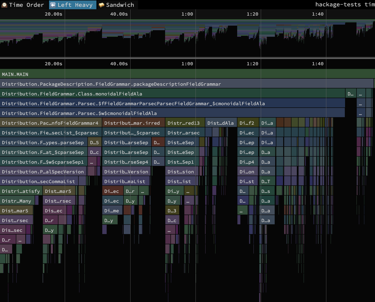
This is the “Left Heavy” view of the profile, meaning the total run time of nodes in the call graph is aggregated and sorted in decreasing order from left to right. Therefore, the most time-intensive path in the call graph is the one furthest to the left. These are the calls that we will try to specialize for our first step on the specialization spectrum.
Let’s see which dictionaries are being passed to which functions most often by
instrumenting Cabal-syntax with the Specialist plugin
and running the specialyze rank command on an event log of the benchmark. Here
are the top five entries in the ranking:
* Distribution.Compat.Parsing.<?> (src/Distribution/Compat/Parsing.hs:221:3-31)
    called 3703 times with dictionaries:
      Distribution.Parsec.$fParsingParsecParser (src/Distribution/Parsec.hs:159:10-31) (Parsing m)
* Distribution.Compat.CharParsing.satisfy (src/Distribution/Compat/CharParsing.hs:154:3-37)
    called 1850 times with dictionaries:
      Distribution.Parsec.$fCharParsingParsecParser (src/Distribution/Parsec.hs:168:10-35) (CharParsing m)
* Distribution.Compat.Parsing.skipMany (src/Distribution/Compat/Parsing.hs:225:3-25)
    called 1453 times with dictionaries:
      Distribution.Parsec.$fParsingParsecParser (src/Distribution/Parsec.hs:159:10-31) (Parsing m)
* Distribution.Compat.CharParsing.char (src/Distribution/Compat/CharParsing.hs:162:3-24)
    called 996 times with dictionaries:
      Distribution.Parsec.$fCharParsingParsecParser (src/Distribution/Parsec.hs:168:10-35) (CharParsing m)
* Distribution.Compat.CharParsing.string (src/Distribution/Compat/CharParsing.hs:182:3-30)
    called 572 times with dictionaries:
      Distribution.Parsec.$fCharParsingParsecParser (src/Distribution/Parsec.hs:168:10-35) (CharParsing m)
...
All of these dictionaries are for the same ParsecParser type. Furthermore,
each of these bindings are actually class selectors coming from the Parsing
and CharParsing classes. The Parsing class is a superclass of
CharParsing:
class Parsing m => CharParsing m where
  ...
By cross-referencing the ranking with the flame graph above, we can see that the
branch of the call graph which care to specialize mostly consists of calls which
are overloaded in either the Parsec or CabalParsing classes. Parsec is a
single-method type class, whose method is itself overloaded in CabalParsing:
class Parsec a where
  parsec :: CabalParsing m => m a
And CabalParsing is declared like this:
class (CharParsing m, MonadPlus m, MonadFail m) => CabalParsing m where
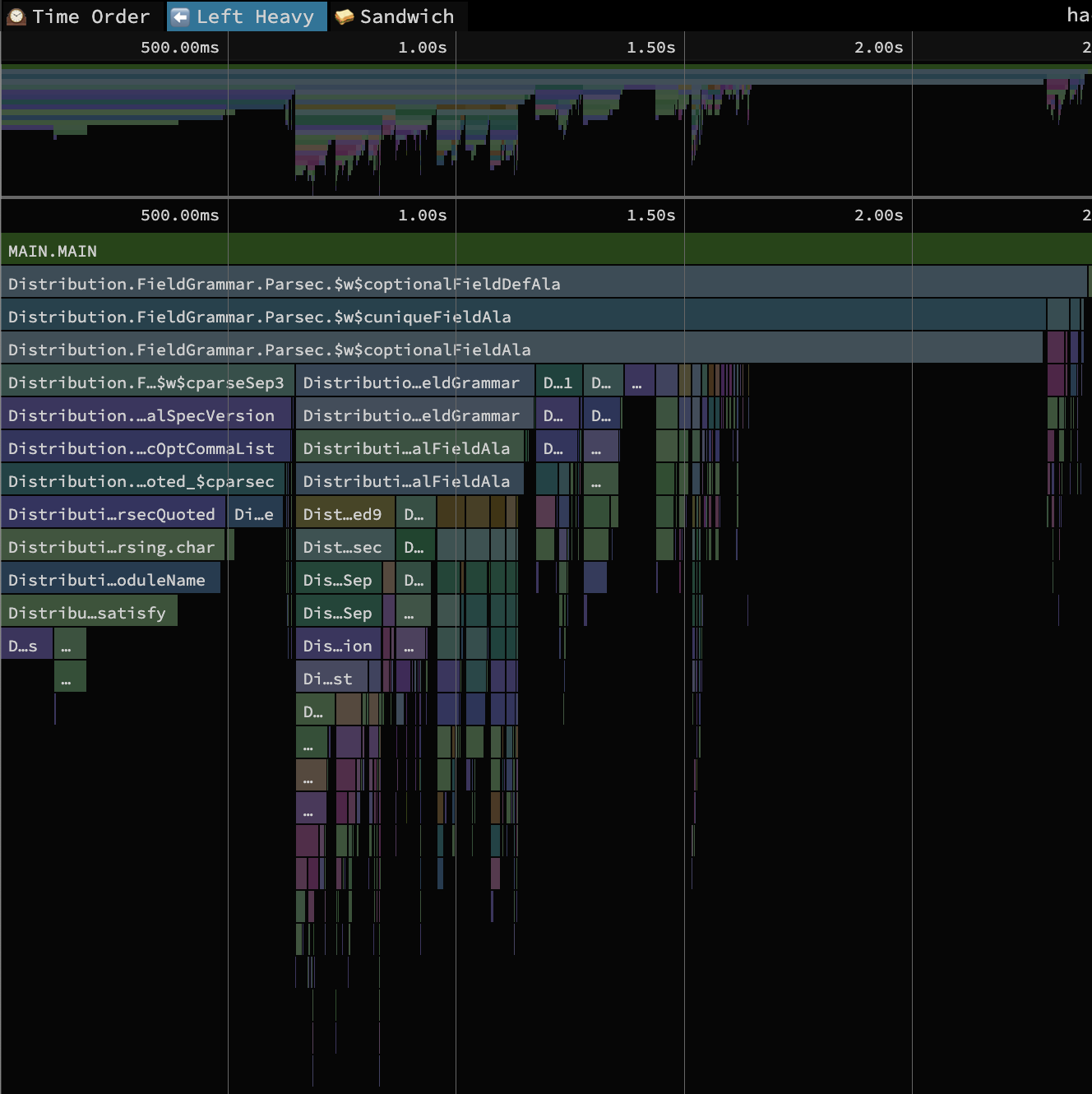
...To take our first step on the specialization spectrum, we can simply walk up the furthest left path in the call graph above and specialize each of the bindings to whichever type/dictionary it is applied at based on the rank output. This is what we have done at this commit on my fork of Cabal. With those changes the entire leftmost overloaded call chain in the flame graph above disappears. Rerunning the benchmarks with profiling enabled, this is the new flame graph we get:
This is what the specialization spectrum looks like at this step:
| Metric | Baseline | Max specialization | Step 1 | Step 1 change w.r.t. baseline |
|---|---|---|---|---|
| Code size | 21,603,448 | 26,824,904 | 22,443,896 | +3.9% |
| Compilation allocation | 111,440,052,583 | 138,939,052,245 | 118,783,040,901 | +6.6% |
| Compilation max residency | 326,160,981 | 475,656,167 | 340,364,805 | +4.4% |
| Compilation time | 40.8 | 52.9 | 44.2 | +8.5% |
| Execution allocation | 688,861,119,944 | 663,369,504,059 | 638,026,363,187 | -7.4% |
| Execution max residency | 991,634,664 | 989,368,064 | 987,900,416 | -0.38% |
| m/s per file | 0.551 | 0.546 | 0.501 | -9.2% |
This is certainly an improvement over the baseline and we have avoided the compilation cost and code size overhead of max specialization.
At this point, we have taken an earnest step on the specialization spectrum and
improved the program’s performance by doing nothing but adding some precise
SPECIALIZE pragmas. If we wanted even better performance,
we could repeat this process for the next most expensive branch of our call
graph above.
Other possible improvements
While writing the SPECIALIZE pragmas for this step, it became clear that we
could avoid most of the overhead resulting from overloaded calls in this code by
manually specializing the parsec method of the Parsec class, rather than
achieving the specialization via SPECIALIZE pragmas. Here is the Parsec
class declaration again:
class Parsec a where
  parsec :: CabalParsing m => m a
The Specialist data, it is obvious that
the only dictionary provided for this constraint is the CabalParsing ParsecParser dictionary. So, we can easily manually specialize all calls to
parsec by changing the class:
class Parsec a where
  parsec :: ParsecParser a
Furthermore, the only CabalParsing instance defined in Cabal is the one for
ParsecParser, so we could further refactor to monomorphize any bindings that
are overloaded in CabalParsing and remove the CabalParsing class altogether.
This is what we did at this commit on my fork of
Cabal. This results in a ~30%
reduction in parse times per file and a ~20% reduction in total allocations,
relative to baseline:
| Metric | Baseline | Max specialization | Step 1 | Specialized parsec |
|---|---|---|---|---|
| Code size | 21,603,448 | 26,824,904 | 22,443,896 | 22,334,736 |
| Compilation allocation | 111,440,052,583 | 138,939,052,245 | 118,783,040,901 | 120,159,431,891 |
| Compilation max residency | 326,160,981 | 475,656,167 | 340,364,805 | 331,612,160 |
| Compilation time | 40.8 | 52.9 | 44.2 | 40.5 |
| Execution allocation | 688,861,119,944 | 663,369,504,059 | 638,026,363,187 | 549,533,189,312 |
| Execution max residency | 991,634,664 | 989,368,064 | 987,900,416 | 986,088,696 |
| m/s per file | 0.551 | 0.546 | 0.501 | 0.39 |
We have proposed this change in this PR on the Cabal repository.
Conclusion
We have covered a lot of ground in this post. Here are the main points:
- Many Haskell programs, especially those in mtl-style, use the
class system for modularity rather than the module system, which makes them
susceptible to very inefficient compilation behavior, especially if
INLINABLEpragmas or-fexpose-all-unfoldingsand-fspecialize-aggressivelyare used. Such methods can result in many useless (i.e. high compilation cost, low performance improvement) specializations to be generated. We should aim to generate only the minimal set of specializations that results in the desired performance. - Careful exploration of the specialization spectrum can help programmers avoid
this undesirable compilation behavior and/or inoptimal performance. We have
developed new tools to help with this.
-fprof-late-overloadedand-fprof-late-overloaded-callsfor getting high-level performance information for the overloaded parts of a Haskell program.- The Specialist GHC plugin for answering very precise, low-level questions about the overloaded parts of a Haskell program.
- These new tools we’ve developed are robust enough to be used on large and complex applications, providing opportunities for significant performance improvements.
Future work
The methods presented in this blog post represent a significant first step towards improving the transparency and observability of GHC’s specialization behavior, but there is still much that can be improved. To further strengthen the analyses we used in this post, we would need a more structured and consistent representation of info table provenance data in GHC. That being said, even without changing the representations, there are some ways that the Specialist plugin and tools could improve (for example) their handling of single-method type class dictionaries.
The ideal conclusion of this kind of work could be an implementation of profile-guided optimization in GHC, where specializations are generated automatically based on previous execution traces made available at compilation. A more difficult goal would be just-in-time (JIT) compilation, where overloaded calls are compiled into specialized calls at run time. Perhaps a more obtainable goal than JIT would be a form of runtime dispatch, where the program could check at runtime if a specific specialization of an overloaded function is available based on the values being supplied as arguments.
Appendix: How to follow along
The examples presented in this post depend on some of the latest and greatest (not yet merged) features of GHC. We encourage interested readers to follow along by building this branch of GHC 9.10 from source.
Footnotes
Later, we will be identifying the exact instances used in overloaded calls based on their source locations stored in the info table map. If we defined these types with
newtype(or usedInt,Double, andIntegerdirectly) instead ofdata, the instances used in the calls would come from modules in thebasepackage. We could still see the exact source locations of these instances using a GHC built with-finfo-table-mapand-fdistinct-constructor-tables; we are simply avoiding the inconvenience of browsingbasemodules for this example by defining our own local types and instances.↩︎The default
duprogram on macOS does not support the-bflag. We recommend using the GNU versiongdu, which is included in thecoreutilspackage on Homebrew and can be installed withbrew install coreutils. You can then replace any invocations ofduin the content above withgdu.↩︎Ticky-ticky profiling is a complex profiling mode that tracks very low-level performance information. As noted in section 8.9.3 of the GHC User’s Guide, it can be used to find calls including dictionary arguments.↩︎
GHC generates names for dictionaries representing instance definitions. These names are typically the class and type names concatenated, prefixed with the string “$f” to make it clear that they are compiler-generated. This name gets put into the info table provenance data (enabled by
-finfo-table-mapand-fdistinct-constructor-tables) for the dictionaries, which is then read by Specialist as a normal identifier.↩︎Unfortunately, as of writing, there is a GHC bug causing some dictionaries to get inaccurate names and source locations in the info table provenance data. In these cases, it can be difficult to link the dictionary information to the actual instance definition. For this reason, we also display the type of the dictionary as determined at compile time, which can be helpful for resolving ambiguity.↩︎
The
--dict MyIntegeroption we specified just tells the tool to only consider samples that include a dictionary (either as a direct argument to the call or as a superclass instance) whose information includes the string “MyInteger”. Therefore, it is important to choose a dictionary string that is sufficiently unique to the instances for the type we are interested in specializing to.↩︎